Table of Contents
Homogeneous Curved Flow
Experiments by Holloway and Tavoularis
Description
These experiments were carried out in order to study the effects of curvature on sheared turbulence in relative isolation from wall and entrainment effects. Uniformly sheared turbulence was allowed to reach a state of transverse statistical homogeneity in a rectangular straight duct and then passed into a curved duct, also of rectangular cross section.
In the experiments, the parameter \(S\) spanned a wide range, from approximately -0.50 to over 1.0, where:
\[ S = \frac{(U_c/R_c)}{dU/dn} \]
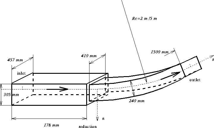
\(U_c\) is the centreline velocity, \(dU/dn\) the mean shear and \(R_c\) the radius of curvature (see figure 1).
3D flow with constant temperature (although for computational purposes the flow can be treated as homogeneous in the cross-stream plane, and thus develops only in the streamwise direction).
Geometry
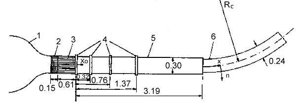
The configuration of experimental apparatus is shown in the sketch in figure 2. For a full description of the wind tunnel at the University of Ottawa refer to Karnik and Tavoularis (1987).
Following a 16:1 contraction (1), the flow passed through a shear generator comprised of 12 separate parallel channels each with a height \(M = 25.4\) mm (2). The next section, the flow separator (3) tended to make the larger scales of the flow uniform. There then followed a straight rectangular test section (5) of height \(h_s = 305\) mm, width 457mm and length 3193mm. The first part of the rectangular section was equipped with four frames, permitting the insertion of grids and screens across the flow (4). The flow then passed through one of two interchangeable curved sections. The curved sections were designed to introduce two distinct degrees of curvature; a mild curvature, which would presumably introduce a small perturbation to the straight shear flow structure and a strong curvature, which would create more profound effects.
As a mild curvature for the flow, a curved section with a centreline radius \(R_c = 5\) m was chosen. As a strong curvature, a section with \(R_c = 2\) m was chosen. The length of the curved sections was chosen with the objective of allowing adequate development of the turbulence, at least for the high-shear cases. In the high shear, straight flow case, the turbulence became self-preserving within 2m of the flow separator for the centreline speeds of interest here. The lengths of the curved sections were therefore chosen to be about 2m. The height, \(h_c\), of the curved sections was 65mm smaller than the height of the upstream straight section and 47mm narrower. The objective of these reductions was to remove the boundary layers built up on the surfaces of the straight section at the entrance to the curved sections, thus reducing the wall effects in the core region of the curved flows.
In order to be able to produce a variety of flow conditions, a combination of three woven screens and one grid of parallel rods was insert into the straight section of the tunnel (4). This produced five sets of flow conditions. Flows with roughly the same magnitudes, but opposite directions of shear were achieved by inverting the shear generator (2), thus giving a total of ten flow conditions.
Flow Characteristics
The flows generated during this experiment displayed two distinct patterns of turbulence development: flows with \(S > 0.05\) had decreasing Reynolds stresses and integral lengthscales, while flows with \(S < 0.05\) had increasing Reynolds stresses and integral length scales. The effect of curvature on the turbulence structure was most clearly displayed by the dimensionless shear stress \(K_{uv}\), which acquired asymptotically constant values when sufficient development time was available. These asymptotic values were monotonically decreasing with increasing \(S\).
According to the authors, in a qualitative sense, the effects of the curvature on the nearly homogeneous shear stress were found to be similar to those observed in curved boundary layers.
Flow Parameters
Air at standard conditions.
Streamwise component of the mean velocity on the wind-tunnel centreline: \(U_c = 10\) m/s.
The curvature parameter is defined as \(S=(U_c/R_c)/(dU/dn)\) where \(n\) is the coordinate normal to the \(s\) coordinate defined along the curved centreline. Six different values of \(S\) are imposed: -0.0079, -0.033, -0.15, 0.032, 0.078 and 0.18.
Inflow Conditions
Experimental values are provided for a flow of equilibrium structure (transverse statistical homogeneity) at \(s = -178\) mm (\(s\) being distance along the tunnel centerline, with \(s=0\) corresponding to the start of the curved section). Six different values of the transverse derivative of the streamwise component of the mean velocity are imposed: \((dU/dn) = -64\) s-1, \(-61\) s-1, \(-31\) s-1, \(30\) s-1, \(64\) s-1 and \(65\) s-1.
For the tunnel centreline (\(n = 0\)), the following quantities upstream of the curved section are available:
- First order moments: \(U\), \(V\), \(W\)
- Second order moments:
- Reynolds stresses: \(\overline{u^2}/k\), \(\overline{v^2}/k\), \(\overline{w^2}/k\), \(\overline{uv}/k\)
- Turbulent kinetic energy: \(k\)
Data is all stored in the file homcurv.dat.
Experimental Details
All measurements were performed with hot-wire anemometers, using a custom made, cross wire array (TSI 1248BJT15). The sensing elements were made of tungsten and had a diameter of 5 \(\mu\)m and a length of 1.2mm. They were separated by 0.5mm and had nominal inclinations of +/-45o with respect to the axis of the probe body.
The hot wires were calibrated in the wind tunnel with all flow obstructions removed to provide a low turbulence airstream.
The sidewalls of the curved sections were engraved with a polar co-ordinate system and the probe tip was positioned by aligning it with the corresponding lines on the two tunnel walls. The axis of the probe body was positioned by eye, tangentially to both the centreplane of the tunnel and the engraved circular co-ordinate at each streamwise location.
The streamwise integral length scales, \(L_{UU}\), \(L_{VV}\) and \(L_{WW}\) were measured by integrating the corresponding autocorrelation coefficients to their first zeros and using Taylor's 'frozen flow' approximation. The streamwise Taylor microscales were measured as:
\[ \lambda_u = \left[ \overline{u^2}/\overline{(\partial u/\partial s)^2} \right]^{1/2} \qquad \lambda_v = \left[ 2\overline{u^2}/\overline{(\partial v/\partial s)^2} \right]^{1/2} \qquad \lambda_w = \left[ 2\overline{u^2}/\overline{(\partial w/\partial s)^2} \right]^{1/2} \]
where the streamwise derivatives were estimated from the corresponding temporal derivatives using Taylor's 'frozen flow' approximation.
Measurement Errors
- \(\delta(\overline{u^2})/\overline{u^2} = 1\%\)
- \(\delta(\overline{v^2})/\overline{v^2} = 2\%\)
- \(\delta(\overline{uv})/\overline{uv} = 5\%\)
Available Measurements
The following measurements are provided at 9 different positions along the tunnel centreline (one location upstream of the curved section, and at \(s/h_c = 0.42\), \(1.25\), \(2.08\), \(2.92\), \(3.75\), \(4.58\), \(5.42\) and \(6.25\)):
- First order moments: \(U\), \(V\), \(W\)
- Second order moments:
- Reynolds stresses: \(\overline{u^2}/k\), \(\overline{v^2}/k\), \(\overline{w^2}/k\), \(\overline{uv}/k\)
- Turbulent kinetic energy: \(k\)
- Streamwise integral length scale
- Taylor's microscale
Sample plots of selected quantities are available.
Mean flow conditions for the cases available:
| \((dU/dn)\) [s-1] | \(S = (U_c/R_c)/(dU/dn)\) | |
|---|---|---|
| \(R_c = 5\) m | -61 | -0.33 |
| 64 | 0.032 | |
| \(R_c = 2\) m | -64 | -0.079 |
| -31 | -0.15 | |
| 65 | 0.078 | |
| 30 | 0.18 |
The data can be downloaded as compressed archives from the links below, or as a single file.
Data for all cases is stored in the file homcurv.dat.
References
- Holloway, A.G.L., Tavoularis, S. (1992). The effects of curvature on sheared turbulence. J. Fluid Mech., Vol. 237, p. 569.
- Holloway, A.G.L., Tavoularis, S. (1991). Effects of curvature on the spectra of sheared turbulence. Proc. 8th Int. Symp. on Turbulent Shear Flows, Munich.
- Karnik, U., Tavoularis, S. (1987). Generation and manipulation of uniform shear with the use of screens. Exp. Fluid, Vol 5, pp. 247-254.
Indexed data:
| case014 (dbcase, free_flow) | |
|---|---|
| case | 014 |
| title | Homogeneous Curved Flow |
| author | Holloway, Tavoularis |
| year | 1990 |
| type | EXP |
| flow_tag | homogeneous, curvature |

