Horizontal Convective Boundary Layer
LES by Schmidt and Schumann
Description
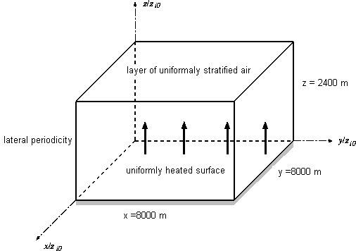
Convective boundary layer in the atmosphere, uniformly heated from below and topped by a layer of uniformly stratified fluid, for zero mean horizontal flow. Results from Large Eddy Simulations.
3D flow with temperature variations.
Geometry of the Domain
The computational domain extends horizontally over a domain of size \(X = 8000\) m (\(= 5z_{io}\)) in the \(x\) and \(y\) directions, and vertically from height \(z = 0\) to \(z = 2400\) m (\(= 1.5z_{io}\)), where \(z_{io}\) is the height of the boundary layer, as shown in figure 1.
Flow Characteristics
The convective boundary layer arises in the atmosphere if the turbulence generated by buoyancy due to upward heat flux from the surface dominates relative to turbulence generated by mean shear. In this case , the convective motion exhibits a coherent structure of convection circulations composed of updraughts and downdraughts. Buoyant updraughts with warm air rising in rather narrow columns are surrounded by larger areas which are slowly sinking as downdraughts.
The computational domain is arranged so that it accommodates several updraughts at a given time, to ensure the lateral periodicity conditions do not significantly influence the results.
Flow Parameters
- Air with a kinematic viscosity \(\nu = 1.5\times 10^5\) m2/s and a density \(\rho = 1.43\) kg/m3.
- Surface normal temperature flux: \(Q_s = 0.06\) K.ms-1.
- Initial constant-temperature of the heated surface: \(T_o = 26.6\)oC.
- Height of the inversion: \(z_i\).
- Height of the boundary-layer: \(z_{io} = 1600\) m.
- Volumetric expansion ratio: \(\beta = 1/300\) K-1.
- Initial convective velocity: \(w^*_o = (\beta gQ_sz_{io})^{1/3} = 1.46\) m/s.
- Temperature scale: \(T^*_o = (Q_s/w^*_o) = 0.041\) K.
Calculated Quantities
For the velocities, the pressure and the temperature, statistical moments, spectra and correlation functions are calculated.
The averaging over an horizontal plane of the quantity \(a\) is denoted \(\langle a \rangle\); and the correlation functions between vertical velocity \(w(x,y,z_c,t)\) at height \(z_c\) and quantity \(f(x+x',y+y',z,t)\) is defined as: \(r_{wf}(x,y,z,t,z_c) = \langle w(x',y',z_c,t)f(x+x',y+y',z,t)\rangle\); with averaging over all positions \((x',y')\) in the domain.
The results presented in Schmidt and Schumann (1989) are compared with some experimental measurements carried out both in laboratory and aboard aircraft.
Simulation Details
Grid
The domain is composed of \(160 \times 160 \times 48\) cubic cells of uniform shape with a side length of 50 m.
Computational Method
The numerical scheme is based on an equidistant staggered grid and finite-difference approximations. The momentum and continuity equations are approximated by second-order central differences in space. The balance equations for the temperature and for the subgrid scale kinetic energy are approximated by a second-order upwind-scheme.
Initial Conditions
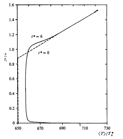
The initial temperature profile of a constant-temperature mixed layer topped by a layer of uniform stability (where \(\partial \theta/\partial z = 0.003\) K/m is set throughout the domain at non-dimensional time \(t^* = 0\) (\(t^* = tw^*_o/z_{io}\)).
At \(t^* = 6\) (\(t = 6575\) s), the mean temperature profile differs from the initial one, as seen in figure 2.
Bottom Surface
The bottom surface is uniformly heated, with an imposed heat flux of \(Q_s\).
Lateral Boundaries
Periodicity is assumed for the four lateral boundaries.
Top Surface
The top surface is part of the uniformly stratified layer. For the horizontal velocity components, free-slip boundary conditions are assumed. The vertical derivative of temperature is prescribed according to the mean temperature profile. The vertical diffusive flux of kinetic energy is set to zero. The pressure and the vertical velocity are connected by means of a radiation boundary condition.
Available Results
Data are provided at three times (\(t^*=6\), \(6.5\) and \(7\)), including:
- Velocity measurements: profiles for \(z/z_{i0}\) up to 1.5 of:
- Second order moments: \(\langle u'^2 \rangle/z_i^{2/3}\), \(\langle w'^2 \rangle/z_i^{2/3}\)
- Dissipation rate of the turbulent kinetic energy: \(\langle \varepsilon\rangle\)
- Third order moments: \( \langle w'^3\rangle/z_i\)
- Skewness: \(S_w\)
- Temperature measurements: profiles for \(z/z_{io}\) up to 1.5 of:
- First order moment: \(\langle T \rangle\)
- Second order moments: \(\langle t'^2\rangle z_i^{2/3}\), \(\langle w'\theta' \rangle\)
- Normalized horizontal spectra of velocities and temperature
Sample plots of selected quantities are available.
The data can be downloaded as compressed archives from the links below, or as individual files.
| \(t^*=6\) | \(t^*=6.5\) | \(t^*=7\) | |
|---|---|---|---|
| File | cbl-data-kp60.dat | cbl-data-kp65.dat | cbl-data-kp70.dat |
Main References
- Schmidt, H., Schumann, U. (1989). Coherent structure of the convective boundary layer derived from large-eddy simulations. J. Fluid Mech., Vol. 200, p. 511.
- Schumann, U. (1989). Large-eddy simulation of turbulent diffusion with chemical reactions in the convective boundary layer. Atmospheric Environment, Vol. 23, pp. 1713.
- Gerz, T., Schumann, U., Elghobashi, S.E. (1989). Direct numerical simulation of stratified homogeneous turbulent shear flows. J. Fluid Mech., Vol. 200, p. 563.
Indexed data:
| case016 (dbcase, semi_confined_flow) | |
|---|---|
| case | 016 |
| title | Horizontal Convective Boundary Layer |
| author | Schmidt, Schumann |
| year | 1988 |
| type | LES |
| flow_tag | scalar, buoyant, 2dbl |

