Wall-Mounted 2-D Hump with Oscillatory Zero-Mass-Flux Jet or Suction through a Slot
Experiments by Greenblatt, Paschal, Yao, Harris, Schaeffler and Washburn
Description
The case is a wall-mounted Glauert-Goldschmidt type body, geometrically similar to that employed by Seifert and Pack (2002). Full details of the current case are given in Greenblatt et al (2004, 2005) and Naughton et al (2004). The model is mounted between two glass endplate frames, as shown in figure 1, and both leading edge and trailing edges are faired smoothly with a wind tunnel splitter plate. This is a nominally two-dimensional experiment, although there are some side-wall effects (3-D flow) near the end-plates. The tunnel dimensions at the test section are 28 inches wide by 20 inches high, but the hump model is mounted on a splitter plate (0.5 inches thick), yielding a nominal test section height of 15.032 inches (distance from the splitter plate to the top wall). The splitter plate extends 76.188 inches upstream of the model's leading edge. Also, 44.437 inches downstream of the model's leading edge, the splitter plate is equipped with a flap (3.75 inches long), which is deflected up during the experiment in order to control the air flow beneath the splitter plate. This control affects the stagnation point at the leading edge of the splitter plate, avoiding massive separation in that region.
 Fig. 1: Hump model and schematic
The characteristic reference length of the model is defined here as the length of the bump on the wall, 16.536 inches. In Seifert and Pack's original work on the hump model, the reference length was defined as the airfoil chord length of 7.874 inches (\(x = 0.0\) to \(x = 7.874\) inches). Their leading edge was then faired smoothly into the wall from \(x = -.3937\) to \(x = .3937\) inches; however this additional length ahead of \(x = 0.0\) was not accounted for in their definition of the reference length. For the current experiment it was felt to be more straightforward to use the actual bump length as the reference length. As a result of this, the current scaled (nondimensional) coordinates of the overall body shape are slightly different from those of Seifert and Pack. A simple rescaling operation can recover it.
The model itself is 23 inches wide between the endplates at both sides (each endplate is approximately 9.25 inches high, 34 inches long, and 0.5 inches thick with an elliptical-shaped leading edge). The model is 2.116 inches high at its maximum thickness point. Both uncontrolled (baseline) and controlled flow scenarios are considered under the conditions of \(M = 0.1\) and \(Re\) somewhat less than 1 million per chord. The tunnel medium is air at sea level. The model experiences a fully-developed turbulent boundary layer whose delta (thickness) at the leading edge of the model is between 1 - 2 inches. The boundary layer is subjected to a favourable pressure gradient over the front convex portion of the body and separates over a relatively short concave section in the aft part of the body, as shown in the 2D CFD results in figure 2. A slot at approximately the 65% chord station on the model extends across the entire span of the hump. Flow control is supplied by means of this two-dimensional slot across the span, immediately upstream of the concave surface. One type of control uses steady suction, which is driven by a suction pump with the mass flow monitored.
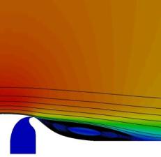 Fig. 2: Sample CFD results for no-control-flow case
For the oscillatory test, separation control is performed using zero efflux oscillatory blowing introduced from the spanwise slot, where careful attention is paid to maintaining slot two-dimensionality. This is achieved by means of a rigid piston that spans the model. The piston is secured to a flange by means of a flexible membrane and the flange is bolted to the base of the plenum. The piston is driven externally by six voice-coil-based actuator modules (Kiedaisch, Nagib and Associates, IIT), generating slot velocities up to 80 m/s at frequencies ranging from 60 Hz to 500 Hz. Schematic views of the assembly from the side and underside of the model (the latter with three modules removed for purposes of illustrating the piston and membrane) are shown in figure 3. A photograph of the underside of the model, prior to tunnel installation, is shown in figure 4. The slot-flow is calibrated and characterized for both tunnel flow-off (quiescent) and flow-on (non-quiescent) conditions, using hot-wire anemometry, throat dynamic pressure measurements and two-dimensional PIV.
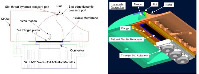 Fig. 3: Schematic of hump model with piston, side view (left) and bottom view (right)
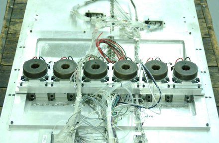 Fig. 4: Photograph of piston assembly
Note that the two endplate frames create blockage which affects all the measurements for this case. See “Experimentalist's Note 3”, in the Experimental Data section below. Also, one of the questions in the FAQS in the Previous Solutions section below addresses this issue.
Flow Details
Flow Conditions
Relevant details for the case are given below. The atmospheric conditions varied, but were essentially standard atmospheric conditions at sea level in a wind tunnel vented to the atmosphere, in a temperature-controlled room.
- \(P_{ambient} \approx 101325\) kg/(ms2)
- \(T_{ambient} \approx 298\) K
- \(\rho_{ambient} \approx 1.185\) kg/m3
- \(\mu_{ambient} \approx 18.4\times 10^{-6}\) kg/(ms)
- \(U_{freestream} \approx 34.6\) m/s
- \(Re_{freestream} \approx 2.23\times 10^6\) per metre, or approx \(9.36\times 10^5\) per chord length of hump
- \(M_{freestream} = 0.10\)
There are three conditions for the case:
- Condition 1: no flow control (no flow through the 23-inch-span slot; slot left open with no suction or blowing through it).
- Condition 2: suction rate of 0.01518 kg/s (27.13 CFM) through the 23-inch-span slot.
- Condition 3: zero-net-mass-flux oscillatory suction/blowing, frequency = 138.5 Hz, peak velocity out of slot during blowing part of the cycle \(U_{jetmax} = 26.6\) m/s. This condition corresponds to an oscillatory blowing momentum coefficient of approximately \(c_{\mu} = \langle J\rangle/(cq) = \rho h(U_{jetrms})^2/(0.5c\rho_{inf}U_{inf}^2) = 0.111\)%, where \(h\) is the slot width.
The upstream boundary conditions from the experiment (associated with the boundary layer on the plate at location \(x/c=-2.14\) upstream of the start of the hump, where \(c = 16.536\) inches \(= 0.4200\) m), to be used to help set/verify inflow BC's, are given in the files below. Note that the oscillatory suction/blowing case used a different unit underneath the splitter plate, feeding into the slot. As a result, the blockage beneath the splitter plate was different, which slightly affected the incoming flow field above the plate. Thus, the boundary layer thickness at \(x/c=-2.14\) for the oscillatory case was slightly smaller than for the no-flow and steady suction cases, and the inlet boundary condition files for this case are given separately in the table below.
| No control flow and suction cases | Oscillatory suction/blowing | |
|---|---|---|
| Mean velocity | case3_pitot_inflow_stats.dat | case3_pitot_inflow_stats_osc.dat |
| Streamwise turbulence intensity | uprime_hw.dat | uprime_hw_osc.dat |
To complete the Reynolds stress matrix for the upstream BC's at \(x/c=-2.14\) it is suggested one can assume incompressible fully-developed boundary layer distributions.
Flow Geometry
This is a nominally two-dimensional experiment, although there will be side-wall effects (3-D flow) near the end-plates. The tunnel dimensions at the test section are 28 inches wide by 15.032 inches high (distance from the splitter plate to the top wall). The model itself spans almost the entire 28-inch tunnel (it is not sealed at the walls), but two endplates are attached to the model, 23 inches apart. The boundary-layer-control slot is located only over the 23-inch hump section between the endplates. Each endplate is approximately 0.5 inch thick, 9.25 inches high, and 34 inches long (see Special Note below). Each endplate has an elliptical-shaped leading edge, at an \(x\) location of 8.48 inches upstream of the start of the hump. A number of sketches and views of the model geometry are shown in figure 5.
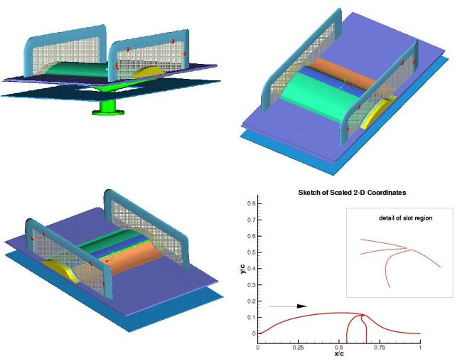 Fig. 5: Views and sketches of the model hump geometry
Some geometry-related data files can be downloaded from the Available Data section below.
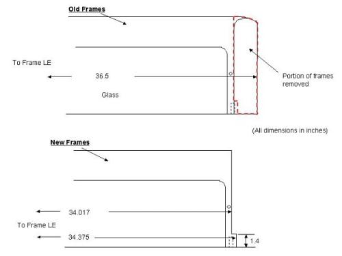
SPECIAL NOTE: Due to limited optical access, it was necessary to modify the downstream portion of the end-plates (by removing some of the frame). This modification, made to both of the end-plates, is illustrated in figure 6. This change is not reflected in any of the other figures above or in the geometry files.
Available Data
The data available includes details of the geometry, pressure and velocity measurements for all three cases (no flow control, suction control and oscillatory control), and sample grids.
Sample plots of selected quantities are available.
The data files can be downloaded as compressed archives, or individually from the descriptions and tables below.
Geometry Data
The table below gives five case geometry-related items.
| File | Contents |
|---|---|
| simplifiedhumpgeom.igs | CAD file in IGES format |
| proefiles.tar.gz | CAD files in ProE (ProEngineer 2001) format |
| qa_compare.tar.gz | Comparisons between theoretical geometry and the actual (QA) geometry |
| coords.dat | 2-D hump coordinates (in inches) |
| coordsnondim.dat | Nondimensionalized 2-D hump coordinates (scaled so that chordlength=1) |
Note that the IGES file does not include the parts of the hump outside of the end-plates (the yellow parts in the figures above). These outside parts are the same hump shape, but there is no slot present for suction/blowing (the slot has been faired over).
Note also that the geometry information is based on theoretical (planned, blueprint-type) specifications. The QA data is given to show differences between the theoretical and as-built configurations. Also, this geometry (specifically the chamber and pipe beneath the splitter-plate floor of the hump model) is used for the suction and no-flow cases. The oscillatory suction/blowing case(s) use a 2D piston-like actuator.
Flow Data
The experimental data are reported in the following coordinate system: \(x\)-direction downstream, \(y\)-direction up, \(z\)-direction spanwise. The coordinate system's origin (0,0,0) is on the tunnel splitter plate at the start of the hump, on the model centreline.
Inflow Data
| Steady cases | Oscillatory suction/blowing | |
|---|---|---|
| Mean velocity | case3_pitot_inflow_stats.dat | case3_pitot_inflow_stats_osc.dat |
| Streamwise turbulence intensity | uprime_hw.dat | uprime_hw_osc.dat |
Steady No-Flow-Control and Suction Experimental Data
Surface Pressure Coefficients
| No-Flow-Control Case | Steady-Suction Control Case | |
|---|---|---|
| Streamwise \(C_p\) profile | noflow_cp.dat | suction_cp.dat |
| Spanwise \(C_p\) profiles | noflow_aux1.dat | suction_aux1.dat |
Note: possible blockage effects in the experiment are not accounted for in this data. The pressure coefficients are all referenced to upstream “freestream” conditions, near \(x/c=-2.14\). The definition of pressure coefficient is \(Cp=(P-P_{ref})/(0.5\rho_{ref} U_{ref}^2)\).
Skin Friction Coefficients
\(C_f\) data (from oil-flow) are available only for the no-flow-control condition
| No-flow-control skin friction | noflow_cf.dat |
The flow reattachment location was \(x/c=1.11 \pm 0.003\) for the no-flow-control condition, and \(x/c=0.94 \pm 0.005\) for the suction condition.
Velocity profiles
Mean velocity components obtained using stereo-PIV at \(x/c=1.0\), \(1.1\), \(1.2\), and \(1.3\) for both no-flow-control and steady-suction conditions. The files below are in the spiv_data of the downloadable archives and contain profiles across the mid-section of these planes (where the flow is essentially 2D), and data covering the whole of each plane.
The file readme.txt contains details of the files and format.
| No-Flow-Control Case | Suction Control Case | |||
|---|---|---|---|---|
| 2D Averaged Data | Whole Plane Data | 2D Averaged Data | Whole Plane Data | |
| \(x/c=1.0\) | spiv-avgvel-noflow-x1-0.dat | spiv-noflow-x1-0.dat | spiv-avgvel-suck-x1-0.dat | spiv-suck-x1-0.dat |
| \(x/c=1.1\) | spiv-avgvel-noflow-x1-1.dat | spiv-noflow-x1-1.dat | spiv-avgvel-suck-x1-1.dat | spiv-suck-x1-1.dat |
| \(x/c=1.2\) | spiv-avgvel-noflow-x1-2.dat | spiv-noflow-x1-2.dat | spiv-avgvel-suck-x1-2.dat | spiv-suck-x1-2.dat |
| \(x/c=1.3\) | spiv-avgvel-noflow-x1-3.dat | spiv-noflow-x1-3.dat | spiv-avgvel-suck-x1-3.dat | spiv-suck-x1-3.dat |
Velocity and turbulence data
Obtained using 2D-PIV along the tunnel centre-plane, roughly covering the region \(0.63 < x/c < 1.39\) for both no-flow-control and steady-suction conditions.
The files below (in Tecplot format) are available in the 2dpivnew directory of the downloadable archives, and cover the area mentioned above, split into four sub-regions (as shown in figure 7).
| Flow Region | No-Flow-Control Case | Suction Control Case |
|---|---|---|
| Region 1 | piv_noflow_1all.dat | piv_suck_1all.dat |
| Region 2 | piv_noflow_2all.dat | piv_suck_2all.dat |
| Region 3 | piv_noflow_3all.dat | piv_suck_3all.dat |
| Region 4 | piv_noflow_4all.dat | piv_suck_4all.dat |
The file readme.txt contains details of the files and format.
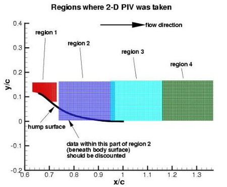 Fig. 7: Regions where 2D-PIV were taken for no-flow and suction conditions
For convenience, extracted and nondimensionalized mean velocity and turbulence profiles (from the files above) at selected \(x/c\) stations for both no-flow-control and steady-suction conditions are given in the files below (located in the extract_2dpivnew directory of the downloadable archives.
| Location | No-Flow-Control Case | Suction Control Case |
|---|---|---|
| \(x/c=0.65\) | x065off.dat | x065on.dat |
| \(x/c=0.66\) | x066off.dat | x066on.dat |
| \(x/c=0.8\) | x080off.dat | x080on.dat |
| \(x/c=0.9\) | x090off.dat | x090on.dat |
| \(x/c=1.0\) | x100off.dat | x100on.dat |
| \(x/c=1.1\) | x110off.dat | x110on.dat |
| \(x/c=1.2\) | x120off.dat | x120on.dat |
| \(x/c=1.3\) | x130off.dat | x130on.dat |
The file readme.txt contains details of the files and format.
Unsteady Oscillatory-Control Synthetic Jet Experimental Data
The time at which peak BLOWING velocity was measured OUT of the slot corresponds to approximately the phase angle of 170o.
Note: The oscillatory-control synthetic jet condition used a different unit (“synthetic jet unit”) underneath the splitter plate, feeding into the slot (as opposed to the “suction unit” used for the original no-flow-control and steady-suction conditions reported above). As a result, the blockage beneath the splitter plate was different, which slightly affected the incoming flow field above the plate.
Mean-flow quantities and turbulence data with no flow control applied were therefore re-taken with the “synthetic jet unit” in place; these are given in Tecplot format in the file baseline_synthunit.dat with in the 2dpivsynthunit directory. The \(C_p\) values for no-flow-control were also re-taken with the “synthetic jet unit” in place; these are given in the file noflow_synthunit_cp.dat. These \(C_p\) data are compared with the no-flow \(C_p\) data using the original “suction unit” in figure 8, showing only very small differences.
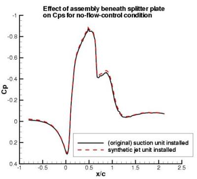 Fig. 8: Effect of assembly beneath splitter plate on no-flow-control condition
Cp data
\(C_p\) data is available in three files, from the table below.
| Data File | Description |
|---|---|
| osccontrol_cpnew.dat | Long-time mean \(C_p\) along the geometry |
| osccontrol_cpphase_mean.dat | Phase-averaged \(C_p\) at 20 positions along the geometry |
| osccontrol_cpphase.dat | Phase-averaged \(C_p\) at 20 positions along the geometry, with mean values subtracted off |
Note: possible blockage effects in the experiment are not accounted for in this data. The pressure coefficients are all referenced to upstream “freestream” conditions, near \(x/c=-2.14\). The definition of pressure coefficient is \(Cp=(P-P_{ref})/(0.5\rho_{ref} U_{ref}^2)\).
2D-PIV data
Velocity and turbulence data are available along the tunnel centreline, as detailed below.
Phase averaged data (in steps of 10o phase angle) covering the four regions shown in figure 9 are available in the files below (files are in Tecplot format).
| Region | Datafile | Readme file | Directory in the downloadable archives |
|---|---|---|---|
| Region 1 | frame1.dat | readme.txt | phasepivdata1 |
| Region 2 | frame2.dat | readme.txt | phasepivdata2 |
| Region 3 | frame3.dat | readme.txt | phasepivdata3 |
| Region 4 | frame4.dat | readme.txt | phasepivdata4 |
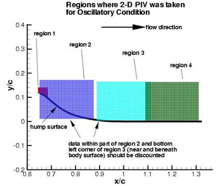 Fig. 9: Regions where 2D-PIV were taken for oscillatory condition
Region 1 is a high resolution data set covering the immediate area near the slot exit. This high quality data set is able to show fine details of flowfield separation due to its high magnification.
Region 2 is a lower resolution data set that overlaps part of Region 1. The differences seen between Regions 1 and 2 are due not only to resolution differences but also to Region 2 imaging problems, near the wall, from \(x/c=0.65\) to \(0.76\). In this \(x/c\) range Region 2 mean velocity is within 20% or better compared with Region 1 data and within 33% in rms velocity for the following phases: 000-020, 080, 110, 130-230, 250-340 (other phases in the Region 2 dataset are less accurate). In figure 10 a typical comparison between Region 1 and Region 2 data at a common station within the range from \(x/c=0.65\) to \(0.76\) is shown.
In Regions 3 and 4, an independent comparison of the 2D PIV data with hotwire data and 3D PIV data showed agreement within 2-3% in the mean at \(x/c=1.3\). The \(u_{rms}\) measurements at \(x/c=1.3\) agreed within the estimated statistical convergence band of 16%. Therefore the PIV measurements in Regions 3 and 4 are estimated to be accurate to within these amounts.
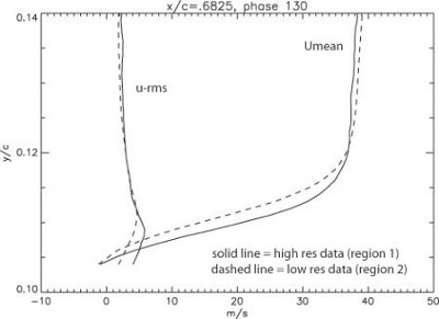 Fig. 10: Sample comparison between region 1 and 2 data
For convenience, nondimensionalized phase-averaged velocity and turbulence profiles have been extracted from the above files at selected \(x/c\) stations at 4 different phase angles in the cycle, as detailed in the table below. These files are in the directory extract_osc_2dpiv.
| Phase Angle | File |
|---|---|
| 80o | expextract.pro.oscphase080.dat |
| 170o | expextract.pro.oscphase170.dat |
| 260o | expextract.pro.oscphase260.dat |
| 350o | expextract.pro.oscphase350.dat |
The file readme.txt give details of the file content and format.
Experimentalist's Notes and Additional Data
Some informal notes and figures (for information only) are provided in the following:
- Microsoft PowerPoint file: data_summary.ppt
- For the interested investigator, additional suction \(C_p\) data at different suction levels are given in the following files:
- suction_cp_00528.dat - streamwise surface pressure coefficients for lower suction condition (\(\dot{m} = .00528\) kg/s).
- suction_cp_00844.dat - streamwise surface pressure coefficients for lower suction condition (\(\dot{m} = .00844\) kg/s).
- suction_cp_02627.dat - streamwise surface pressure coefficients for higher suction condition (\(\dot{m} = .02627\) kg/s).
- As discussed elsewhere, throughout the entire experiment, endplates (positioned on both sides of the model near the side walls) were employed to improve the two-dimensionality of the flowfield. However, they also had a blockage effect. The effect of the endplates on the centreplane streamwise surface pressure coefficient (no-flow condition) can be seen in figure 11, which plots the standard result (with endplates) against the result when the endplates were temporarily removed (noflow_cp_noplates.dat).
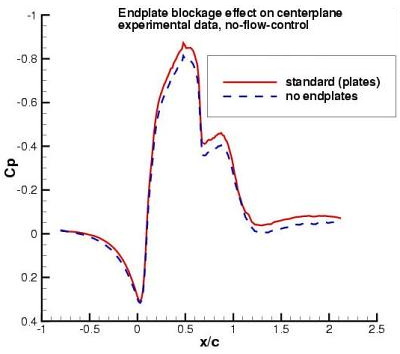 Fig. 11: Effect of endplates on Cp, no-flow
- An Excel file summarizing \(C_p\) and \(C_{p-rms}\) data with the synthetic jet unit in place is given in datasummaryzeojetcfd.xls.
- Two .avi movie files illustrate the oscillatory condition flowfield:
- case3_vector.avi - movie file (.avi format) showing velocity vectors.
- dynamicpressures.avi - movie file (.avi format) showing phase-averaged surface pressure coefficients (with mean \(C_p\) subtracted).
- Two Excel files of data for the oscillatory condition, giving systematic variation of \(C_p\) data with frequency and peak slot velocity:
- cpdatapeakvelocity.xls - Excel file giving mean and phase-averaged \(C_p\) for various peak velocities at a given frequency \(f=138.5\) Hz.
- cpdatafrequency.xls - Excel file giving mean and phase-averaged \(C_p\) for various frequencies at a given peak slot velocity \(V_{out}=26.6\) m/s.
Grids
These grids are provided in case computors want or need one, or need a starting-off point for developing their own grids. Note that these grids were created with RANS in mind. However, there is no guarantee that they are free from defects, or that they possess adequate grid spacing. Also, the grids have a “farfield” extent that may, or may not, be sufficient for all codes and/or flow conditions.
Structured 2-D Grids
Structured 2D Grid #1: 4-zone point-matched (nondimensional with respect to chord of 16.536 inches) (210,060 grid points total) in PLOT2D format. Source: C. Rumsey (NASA LaRC).
| case3-struct-1-p2dfmt.gz | gzipped grid (2.9 MB) |
| case3-struct-1-roadmap.txt | description of the grid system |
Note that grid zone 4 extends forward to \(-6.39c\), which was found in preliminary CFD tests to yield a “run” long enough so that the computed boundary layer thickness approximately matches that of experiment. This forward extent is longer than the actual splitter plate length. Also note that the top tunnel wall uses inviscid-type grid spacing, which may or may not be appropriate.
Structured 2D Grid #2: same grid as #1, but coarser (every other point in each coordinate direction) (52,952 grid points total) in PLOT2D format. Source: C. Rumsey (NASA LaRC).
| case3half-struct-1-p2dfmt.gz | gzipped grid (0.7 MB) |
| case3half-struct-1-roadmap.txt | description of the grid system |
Note that grid zone 4 extends forward to \(-6.39c\), which was found in preliminary CFD tests to yield a “run” long enough so that the computed boundary layer thickness approximately matches that of experiment. This forward extent is longer than the actual splitter plate length. Also note that the top tunnel wall uses inviscid-type grid spacing, which may or may not be appropriate.
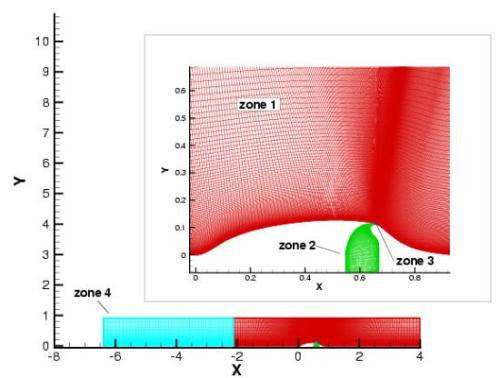 Fig. 12: View of structured grid 1
Structured 2D Grid #3 (No Slot): 1-zone (nondimensional with respect to chord of 16.536 inches) (143,613 grid points total) in PLOT2D format. Source: C. Marongiu (CIRA - Italian Aerospace Research Center).
| case3-struct-3-p2dfmt.gz | gzipped grid (1.2 MB) |
Note that this grid fairs over the slot, as shown in figure 13. Upstream extent is \(x/c=-2.14\), downstream extent is \(x/c=4.0\). Top wall is at \(y/c=0.909\).
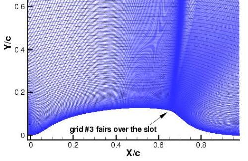 Fig. 13: View of structured grid 3 around the hump
Structured 2D Grid #4: 4-zone point-matched, with top wall shape adjusted to approximately account for side plate blockage (see figure 14). All dimensions are nondimensional with respect to chord of 16.536 inches (210,060 grid points total) in PLOT2D format. Source: C. Rumsey (NASA LaRC).
| case3-struct-4-p2dfmt.gz | gzipped grid (2.8 MB) |
| case3-struct-4-roadmap.txt | description of the grid system |
| newtop.dat | file containing approximated top-wall adjusted points |
Note that grid zone 4 extends forward to \(-6.39c\), which was found in preliminary CFD tests to yield a “run” long enough so that the computed boundary layer thickness approximately matches that of experiment. This forward extent is longer than the actual splitter plate length. Also note that the top tunnel wall uses inviscid-type grid spacing, which may or may not be appropriate.
Structured 2D Grid #5: same grid as #4, but coarser (every other point in each coordinate direction) (52,952 grid points total) in PLOT2D format. Source: C. Rumsey (NASA LaRC).
| case3half-struct-4-p2dfmt.gz | gzipped grid (0.7 MB) |
| case3half-struct-4-roadmap.txt | description of the grid system |
Note that grid zone 4 extends forward to \(-6.39c\), which was found in preliminary CFD tests to yield a “run” long enough so that the computed boundary layer thickness approximately matches that of experiment. This forward extent is longer than the actual splitter plate length. Also note that the top tunnel wall uses inviscid-type grid spacing, which may or may not be appropriate.
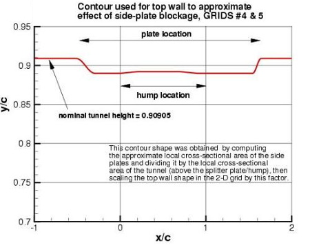 Fig. 14: Depiction of adjusted top wall in grids 4 and 5
The format for the structured 2D grids is PLOT3D-type, formatted, MG, 2D:
  read(2,*) nbl
  read(2,*) (idim(n),jdim(n),n=1,nbl)
  do n=1,nbl
    read(2,*) ((x(i,j,n),i=1,idim(n)),j=1,jdim(n)),((y(i,j,n),i=1,idim(n)),j=1,jdim(n))
  enddo
Unstructured 2-D Grids
Unstructured 2D Grid #1: unstructured grid with upstream extent of \(-6.39c\) (nondimensional with respect to chord of 16.536 inches; 123703 nodes, 368476 faces, and 247404 cells) in FUN2D format. Source: S. Viken (NASA LaRC).
| hump6-39cfine-0-faces.gz | gzipped grid (4.8 MB) |
| case3-unstruct-6-39cfine-roadmap.txt | description of the grid system |
Note that the grid extent of \(-6.39c\) was chosen because it was found in preliminary CFD tests to yield a “run” long enough so that the computed boundary layer thickness approximately matches that of experiment. This forward extent is longer than the actual splitter plate length. Also note that the top tunnel wall uses inviscid-type grid spacing, which may or may not be appropriate.
Unstructured 2D Grid #2: coarser unstructured grid with upstream extent of \(-6.39c\) (nondimensional with respect to chord of 16.536 inches; 57152 nodes, 169689 faces, and 114302 cells) in FUN2D format. Source: S. Viken (NASA LaRC).
| hump6-39ccoarse-0-faces.gz | gzipped grid (2.1 MB) |
| case3-unstruct-6-39ccoarse-roadmap.txt | description of the grid system |
Note that the grid extent of \(-6.39c\) was chosen because it was found in preliminary CFD tests to yield a “run” long enough so that the computed boundary layer thickness approximately matches that of experiment. This forward extent is longer than the actual splitter plate length. Also note that the top tunnel wall uses inviscid-type grid spacing, which may or may not be appropriate.
Unstructured 2D Grid #3: unstructured grid with upstream extent of \(-2.14c\) (nondimensional with respect to chord of 16.536 inches; 116110 nodes, 345880 faces, and 232218 cells) in FUN2D format (use this grid only if you plan to specify boundary conditions directly at the “inflow” location of \(x/c=-2.14\) to match the experiment). Source: S. Viken (NASA LaRC).
| hump2-14cfine-0-faces.gz | gzipped grid (4.5 MB) |
| case3-unstruct-2-14cfine-roadmap.txt | description of the grid system |
Note that the top tunnel wall uses inviscid-type grid spacing, which may or may not be appropriate.
Unstructured 2D Grid #4: coarser unstructured grid with upstream extent of \(-2.14c\) (nondimensional with respect to chord of 16.536 inches; 51546 nodes, 153005 faces, and 103090 cells) in FUN2D format (use this grid only if you plan to specify boundary conditions directly at the “inflow” location of \(x/c=-2.14\) to match the experiment). Source: S. Viken (NASA LaRC).
| hump2-14ccoarse-0-faces.gz | gzipped grid (1.9 MB) |
| case3-unstruct-2-14ccoarse-roadmap.txt | description of the grid system |
Note that the top tunnel wall uses inviscid-type grid spacing, which may or may not be appropriate.
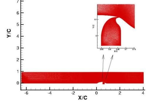 Fig. 15: View of unstructured grid
The format for the unstructured 2D grids is FUN2D-type, formatted:
c There are nfaces jk() arrays (one for each face). Each jk() array contains 2 nodes for the
c face and 2 cells, one on each side of the face.
c
c
      read(2,*)mk,mj,mi0,nsface,nvface,nfface   !nnodes,nfaces,ncells,ninviscidfaces,nviscousfaces,
                                                 !nfarfieldfaces
      read(2,2)((jk(j,l),l=1,4),j=1,mj)         !all the faces jk() array
          ! The line in question reads 2 nodes and 2 cells for each edge/face:
          ! 1st entry is the node on the "left"
          ! 2nd entry is the node on the "right"
          ! 3rd entry is the cell to the left of the edge
          ! 4th entry is the cell to the right of the edge
    2 format(10i12)
c
      if(nsface.gt.0)then                        !actuator and symmetry faces
      read(2,*)
      read(2,2)(isface(j),j=1,nsface)           !isface(j) is the sym. bface index to the jk() array
      endif
c
      if(nvface.gt.0)then
      read(2,*)
      read(2,2)(ivface(j),j=1,nvface)           !ivface(j) is the no-slip bface index to the jk() array
      endif
c
      if(nfface.gt.0)then
      read(2,*)
      read(2,2)(ifface(j),j=1,nfface)           !ifface(j) is the farfield bface index to the jk() array
      endif
c
      read(2,*)
      do 20 k=1,mk
   20 read(2,3)x(k),y(k)
    3 format(2e19.10)
Recommendations and Advice for Calculations
The case has been studied in both the NASA Langley Research Center Workshop on CFD Validation of Synthetic Jets and Turbulent Separation Control in March 2004, and the 11th ERCOFTAC/IAHR Workshop on Refined Turbulence Modelling in April 2005.
A number of answers to frequently asked questions regarding the case were provided for the NASA workshop:
Q: Is there any information available on the boundary layer thickness on the TOP wall (at say, \(x/c=-2.14\))?
A: The top wall boundary layer thickness at \(x/c=-2.14\) was measured (using a pitot probe) to be 0.849 inches when \(U/U_{inf}=0.99\). The corresponding top wall displacement thickness was 0.0866 inches.
Q Is there any boundary layer control being used on the top wall?
A: No.
Q: Is the experimental setup the same as described in the Reno paper AIAA 2003-0218 (Viken et al)?
A: In AIAA 2003-0218, CFD was used to compute the hump model of Seifert and Pack (2002). The current hump model being used in this workshop is a very similarly-shaped model to that used by Seifert and Pack (at a different scale), but it is not identical in all respects. Also, the current test is conducted in a different wind tunnel, and the current model is mounted on a splitter plate.
Q: Are there any mass flow measurements through the channel available?
A: No.
Q: Why are my \(C_p\) values shifted with respect to experiment at all locations (even upstream of the model)?
A: CFD should be expected to agree reasonably well with experimental \(C_p\) levels upstream of the model (e.g., \(-0.8 < x/c < 0\)). Any significant shift in this region may indicate a problem with reference conditions used to process CFD's \(C_p\) data. The reference conditions used in the experiment are upstream of the model, where \(M=0.1\). The definition of pressure coefficient is \(Cp=(P-P_{ref})/(0.5\rho_{ref} U_{ref}^2)\) Basically, what you want in your code is to use the same reference conditions upstream where \(M=0.1\). If you are running one of the “traditional” farfield-type CFD codes, then your Mach number upstream may end up being slightly different from 0.1 and/or \(P_{ref}\) may not correspond with the reference Mach number; and small differences at this low a Mach number translate to significant differences in \(C_p\). Two ways to fix this are: (1) re-process your \(C_p\) levels to use an appropriate reference pressure from upstream, rather than the one chosen by the code at the outflow plane; or (2) adjust the back pressure at the outflow plane so that the correct reference level is achieved in the simulation.
Q: What is the value of \(c_{\mu}\) for the Case 3 suction case?
A: The target \(c_{\mu}\) is 0.242%, which corresponds with the \(c_{\mu}\) from Seifert and Pack (2002) of 0.2545% with the old chord definition (see Case intro page for a discussion on this). So with the new 5% longer chord, target \(c_{\mu}\) for the current test is 0.242%. Note that uncertainties in measuring \(\dot{m}\) get magnified when computing \{c_{\mu}\). So actual \(c_{\mu}\) can vary from test to test by as much as 3-4%. However, this level of uncertainty makes no perceptible difference in the measured results. From the CFD perspective, it is best to try to match the m_dot (0.01518 kg/s) from the experiment.
Q: What is the nominal tunnel “freestream” turbulence level in the 28 x 20 inch tunnel?
A: In previous testing, data were taken with a single normal hot-wire (\(u\) component only) with a bandwidth of 1.56 Hz to 10 kHz. After removing the component that seems to be coming from structural vibration, the Tu level was 0.09% at M=0.1. (The part of the spectra involved in structural vibration was frequencies below 20 Hz. Note, this does not mean that everything below 20 Hz was thrown out; only the portion that correlated with accelerometer measurements was removed.)
Q: Why does the Mach contour plot shown in the logo for Case 3 appear to have a higher freestream Mach number than 0.1?
A: That plot, which has served as part of the logo or “icon” for Case 3 since the beginning (see, for example, the right-hand plot on the home page), is from the paper of Viken et al (AIAA 2003-0218). This paper modelled the Seifert-Pack hump configuration, which was slightly different from the current hump model configuration, and was tested in a different wind tunnel. It used \(M=0.25\), which is higher than the \(M=0.1\) for the Case 3 of the current workshop. Thus, this figure should not be used for quantitative comparison purposes.
Q: Can you explain the splitter plate set-up?
A: An explanation of the wind tunnel and splitter plate set-up can be found in the Case Description above. Also, there is a rough sketch in figure 16 showing some details:
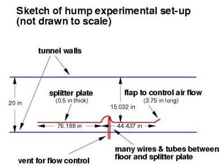 Fig. 16: Sketch of hump wind-tunnel set-up
Q: Is there any dominant frequency present in the unsteady structures of the separated flow?
A: To date, no downstream hotwire data have been taken to answer this question definitively. However, unsteady surface pressure data show no indication of any clear dominant frequency.
Q: What was the reattachment point measured in the experiment?
A: For the no-flow-control case, the oil film technique was used to measure wall shear stress. This technique indicated an approximate mean reattachment point at \(x/c=1.11\). The flow is highly unsteady at reattachment as indicated by the peak in Cp' at this location. The uncertainty associated with this location is \(x/c=1.11 \pm 0.003\). Oil film has also recently been used to determine the reattachment point for the suction case: it is \(x/c=0.94 \pm 0.005\).
Q: Can you describe the piston arrangement for the oscillatory case condition?
A: The piston assembly (or “synthetic jet unit”) is mounted at the bottom of the hump cavity, which extends 1 inch (or \(y/c = 0.06052\)) below the top of the splitter plate floor (as shown under Case Geometry as well as in the supplied grids). The piston itself consists of a solid plate mounted on a flexible membrane, and is driven electro-mechanically. The flexible membrane face is approximately 23 inches wide (in the spanwise \(z\)-direction) by 2 inches long (in the streamwise \(x\)-direction); and the solid plate, approximately centred on the membrane, is approximately 22.53 inches wide (in the spanwise \(z\)-direction) by 1.59 inches long (in the streamwise \(x\)-direction) by about 0.035 inches thick (in the vertical \(y\)-direction). At rest, when the piston assembly is mounted at the bottom of the hump cavity, the flexible membrane is located approximately 1.122 inches below the top of the splitter plate floor, and the piston face is located approximately 1.087 inches below the top of the splitter plate floor. It is important to note that use of the piston assembly (or “synthetic jet unit”) changed the blockage beneath the splitter plate, compared to when the “suction unit” was used for the no-flow-control and steady-suction conditions. As a result, the incoming flow field above the plate was slightly affected. The effect on \(C_p\) was fairly small. See additional discussion under Experimental Data.
Q: For the oscillatory case condition, precisely where and how is the peak velocity out (of 26.6 m/s) being measured?
A: The peak velocity out is being measured at the jet exit approximately along an imaginary line level with the hump surface. The slot is being calibrated (with the tunnel flow off) at the centre-span location on the model. A hot wire will be placed in the “top-hat” region of the (oscillatory) issuing jet, i.e. the constant velocity core region of the jet. Data for a large number of cycles will be acquired and the average of the peaks will be computed. Uncertainty will be given, and sensitivity of the global flowfield to parametric variations in the peak velocity (or \(c_{mu}\) based on rms velocity) will be determined.
Q: How can I account for endplate blockage in my CFD computation?
A: One way to account for endplate blockage is to run the SAME configuration as experiment; this means a 3-D computation, including the endplates inside the tunnel. Alternatively, the endplate blockage can be approximately accounted for in a 2-D computation by (crudely) contouring the tunnel top wall shape to reduce the local tunnel area by an appropriate amount. Note that the endplate blockage issue was not recognized at the time of the workshop (March 2004). Grids have since been created with an adjusted top wall shape, and are available from the Downloads section.
Related Publications
- Greenblatt, D., Paschal, K.B., Yao, C.-S., Harris, J., Schaeffler, N.W., Washburn, A.E. (2004). A Separation Control CFD Validation Test Case, Part 1: Baseline and Steady Suction. AIAA 2004-2220.
- Greenblatt, D., Paschal, K.B., Yao, C.-S., Harris, J. (2005). A Separation Control CFD Validation Test Case, Part 2: Zero Efflux Oscillatory Blowing. AIAA 2005-0485.
- Naughton, J.W., Viken, S.A., Greenblatt, D. (2004). Wall Shear Stress Measurements on the NASA Hump Model for CFD Validation. AIAA 2004-2607.
- Naughton, J.W., Viken, S., Greenblatt, D. (2006). Skin Friction Measurements on the NASA hump model. AIAA Journal, Vol. 44(6), pp. 1255-1265.
- Seifert, A., Pack, L.G. (2002). Active Flow Separation Control on Wall-Mounted Hump at High Reynolds Numbers. AIAA Journal, Vol. 40(7), pp. 1363-1372.
Indexed data:
| case083 (dbcase, confined_flow) | |
|---|---|
| case | 083 |
| title | Wall-mounted two-dimensional hump with oscillatory zero-mass-flux jet or suction through a slot |
| author | Greenblatt, Paschal, Yao, Harris, Schaeffler, Washburn |
| year | 2004 |
| type | EXP |
| flow_tag | 2d, separated, unsteady, varying_cross_section |
