Table of Contents
Upslope and Vertical Convective Boundary Layer
Large Eddy Simulation by Schumann
Description
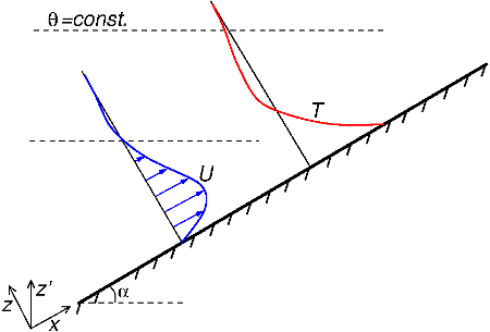
Large-eddy simulation has been used to determine the turbulent structure of the steady-state up-slope boundary layer (UBL) which forms at a uniformly heated inclined or vertical plane surface below a stratified atmosphere at rest. The configuration is shown in figure 1. Data are available for two inclination angles: 10o and 90o.
Simulation Details
The surface plane is inclined by the slope-angle \(\alpha\), as shown in figure 1. The atmosphere above the plane is approximated in the Boussinesq sense, i.e. density \(\rho\) is assumed to be constant except for buoyancy effects. The vertical gradient of potential temperature \(d\theta/dz'\), and the volumetric expansion coefficient \(\beta\), are assumed to be constant. The plane has a rough surface which is characterized by a roughness height \(z_o\), and there is a prescribed kinematic heat flux \(Q_s\) per unit surface area.
From the assumed atmospheric conditions we can define the Brunt-Vaisala frequency \(N=(g \beta\, d\theta/dz')^{1/2}\), and characteristic velocity (\(v^*\)), length (\(H\)) and temperature (\(\theta^*\)) scales can then be defined as \[ v^*= (\beta g Q_s/N)^{1/2} \qquad H=v^*/N \qquad \theta^*=Q_s/v^* \]
In the present study values representative of atmospheric boundary layers have been taken, resulting in \[ N=0.01\text{ s$^{-1}$} \quad v^*=0.58\text{ m/s} \quad H=58\text{ m} \quad \theta^*=0.17\text{ K} \quad z_o=0.2\text{ m} \]
The LES modelling approach used includes a transport equation for the sub-grid-scale kinetic energy, as described in Schmidt and Schumann (1989). The numerical integration scheme is described in Schumann et al. (1987), and employs an equidistant staggered grid and finite difference approximations. The momentum and continuity equations are approximated by second-order central differences in space with the Adams-Bashforth scheme for integration in time. The balance equations for temperature and for SGS kinetic energy are approximated by a second-order upwind scheme.
As explained in Schumann (1990), the flow will reach a steady state, via a series of rather slowly decaying oscillations. To accelerate this process a control scheme was introduced which relaxed the temperature and velocity fields towards the steady state, in order to reduce the required computation time.
Details of domain size (\(X\times Y \times Z\)), grid (\(N_x \times N_y \times N_z\)), time-step (\(\Delta t\)) and total simulation time (\(t_{max}\)) for the two cases considered here are given in the table below.
| Case | \(\alpha\) | \(z_o/H\) | \(X/H\) | \(Y/H\) | \(Z/H\) | \(N_x\) | \(N_y\) | \(N_z\) | \(\Delta t\,N\) | \(t_{max}N\) |
|---|---|---|---|---|---|---|---|---|---|---|
| D10 | 10 | 0.003 | 25.6 | 12.8 | 9.6 | 128 | 64 | 48 | 0.015 | 60 |
| D90 | 90 | 0.003 | 4.8 | 2.4 | 1.8 | 128 | 64 | 48 | 0.0025 | 20 |
In the results, the temperature variable \(T\) denotes departures from the hydrostatic potential distribution.
Available data
Data available includes normalized profiles of flow variables normal to the surface for two cases (\(\alpha=10^o\) and the vertical \(\alpha=90^o\) case). Profiles are provided at a selection of times during the simulation, and the flow quantities reported are:
- Mean velocity and temperature
- Reynolds stresses and turbulent heat flux
Sample plots of selected quantities are available.
The data can be downloaded as compressed archives from the links below, or as individual files.
| Flow quantity | 10o Case | 90o Case |
|---|---|---|
| Mean \(U\) velocity | ubl10um.dat | ubl90um.dat |
| Mean temperature \(T\) | ubl10tm.dat | ubl90tm.dat |
| Streamwise Reynolds stress, \(\overline{u^2}\) | ubl10uu.dat | ubl90uu.dat |
| Transverse Reynolds stress, \(\overline{v^2}\) | ubl10vv.dat | ubl90vv.dat |
| Wall-normal Reynolds stress, \(\overline{w^2}\) | ubl10ww.dat | ubl90ww.dat |
| Reynolds shear stress, \(\overline{uw}\) | ubl10uw.dat | ubl90uw.dat |
| Streamwise turbulent heat flux, \(\overline{ut}\) | ubl10ut.dat | ubl90ut.dat |
| Wall-normal turbulent heat flux, \(\overline{wt}\) | ubl10wt.dat | ubl90wt.dat |
| Turbulent kinetic energy dissipation rate, \(\varepsilon\) | ubl10ep.dat | ubl90ep.dat |
References
- Schumann, U., Hauf, T., Holler, H., Schmidt, H., Volkert, H. (1987). A mesoscale model for the simulation of turbulence, clouds and flow over mountains: Formulation and validation examples. Beitr. Phys. Atmos., Vol. 60, pp. 413-446
- Schmidt, H., Schumann, U. (1989). Coherent structure of the convective boundary layer derived from large-eddy simulations. J. Fluid Mech., Vol. 200, pp. 511-562.
- Schumann, U. (1990). Large Eddy Simulation of the up-slope boundary layer. Quart. J. Roy. Met. Soc., Vol. 116, pp. 637-670.
Indexed data:
| case054 (dbcase, semi_confined_flow) | |
|---|---|
| case | 054 |
| title | Upslope and vertical convective boundary layer |
| author | Schumann |
| year | 1990 |
| type | LES |
| flow_tag | 2d, scalar, buoyant, 2dbl |
