Thermal Boundary Layers in Turbulent Rayleigh-Bénard Convection at Aspect Ratios Between 1 and 9
Experiments by du Puits, Resagk and Thess
Description
Highly resolved temperature measurements are reported in turbulent Rayleigh-Bénard convection in air at a fixed Prandtl number \(Pr = \nu/k = 0.7\) (with \(\nu\)-the kinematic viscosity and \(k\)-the thermal diffusivity). Extending their previous work (du Puits et al, 2007b), the authors carried out measurements at various aspect ratios while keeping the Rayleigh number constant. They demonstrate that the temperature field inside the convective boundary layers of both horizontal plates is virtually independent of the global flow pattern accompanying the variation in the aspect ratio. Thanks to technical upgrades of the experimental facility as well as a significant improvement of the accuracy and reliability of their temperature measurement - and unlike in the previous work - they found that the measured profiles of the time-averaged temperature field neither follow a clear power-law trend nor fit a linear or a logarithmic scaling over a significant fraction of the boundary-layer thickness. Analyzing the temperature data simultaneously acquired at both horizontal plates, various transitions in the cross-correlation and the auto-correlation function of the temperature signals were observed while varying the aspect ratio \(\Gamma = D/H\) (with \(D\) being the lateral dimension of the tank and \(H\) the distance between the hot bottom and the cool top plate). It was suggested that these transitions might be associated with a change in the global flow pattern from a single-roll mode at \(\Gamma = 1\) toward a double- or a multi-roll mode pattern at higher aspect ratios, for more details see du Puits et al (2013).
Experimental details
Experimental facility
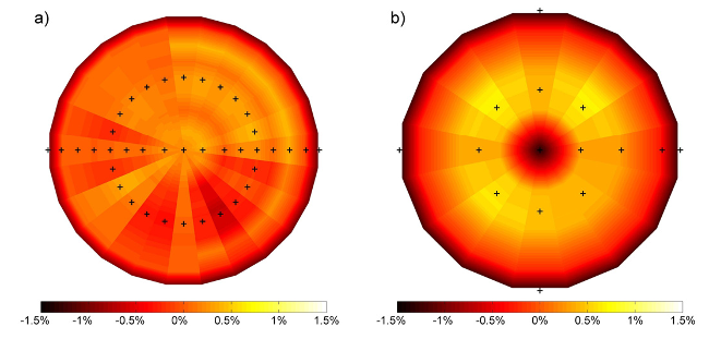
The measurements have been carried out in a cylindrical Rayleigh-Bénard cell of a fixed diameter D = 7.15 m. The working fluid is air with a Prandtl number Pr = 0.7 virtually independent of temperature. The fluid is confined between the heated bottom plate and the free-hanging cooling plate as well as a virtually adiabatic sidewall. The bottom plate actually used in the experiment consists of two parts: an electrical underfloor heating system embedded in a 5 cm concrete layer and isolated from the ground with 0.3 m polyurethane plates and an overlay in which water circulates. The water circulation inside this overlay makes the temperature at the surface of the heating plate uniform and balances the differences of the convective heat flux at the plate-air interface. Both layers are thermally coupled by a 2 mm silicon pad. It is noted here that, compared with previous work published in du Puits et al (2007), the new set-up significantly homogenizes the temperature distribution at the surface of the heating plate (see figure 1). The temperature at the heating plate has been adjusted in a range between \(T_h = 31.2\) and \(58.2^o\)C. The deviation of any local temperature at the surface from the global mean temperature was typically less than +/- 1% of the total temperature drop between the plates (+/- 1.5% at the cooling plate). Over the period of one measurement, the mean surface temperature varies in a band +/- 0.02 K.
 Fig. 1: Temperature distribution at the surface of the heating plate (a) and the cooling plate (b) at Th - Tc = 35.2 K, aspect ratio of 2.75 and Ra = 5.2E10. The plots show the relative deviation ΔTh = 100 [Th(x, y) - Th]/[Th - Tc] and ΔTc = 100 [Tc - Tc(x, y)]/[Th - Tc] as a percentage of the total temperature drop between the plates. The crosses indicate the position of the internal temperature sensors. The radial temperature distribution at each segment is a projection of the measured distribution along the horizontal line, whereas the angular distributed temperature sensors are used as basic values.
The free-hanging cooling plate consists of 16 segments with water circulation inside as well. The segments are mounted on a solid steel construction and are separately levelled perpendicular to the vector of gravity. The entire construction with a weight of about 6 tons is mounted on a crane and can be lifted up and down. A small gap between the plate and the sidewall, required to freely move the plate, is hermetically sealed with strips of foam during the experiments. In the present experiments, the temperature of the cooling plate was set between \(T_c = 28.8\) and \(12.4^o\)C with the same accuracy as indicated for the heating plate. The plate distance has been varied from H = 6.30 m to 0.79 m covering aspect ratios between \(\Gamma = 1.13\) and \(9.00\). The sidewall of the Rayleigh-Bénard cell is shielded by an active compensation heating system to prevent heat exchange with the surroundings. Electrical heating elements are arranged between an inner and an outer isolation of 16 and 12 cm thickness, respectively. The temperature of these elements is controlled to be equal to the temperature at the inner surface of the wall. The heat loss was checked by setting the temperature of both plates to 30.0oC, the fluid temperature that was maintained in the well-mixed bulk region during our experiments. In the case of a perfectly adiabatic side wall, the fluid temperature has to be exactly the same. The measured values were 29.9oC, a deviation that indicates a very small heat loss not exceeding 0.5% of the convective heat flux in the experiments. For more detailed information see du Puits et al (2007a).
Measurement technique
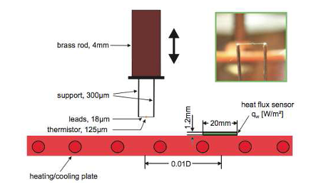
Local temperature measurements have been carried out inside and outside the boundary layers. Here, boundary layers are referred to as those regions where the temperature increases or decreases from the plate temperature to the temperature of the well-mixed core. It should be noted as well that the typical thickness of this region is of the order of 1 cm in the 6.3 m-high Rayleigh-Bénard cell, at the maximum possible Rayleigh number \(Ra = (\beta g \Delta \theta H^3)/(\nu k) = 10^{12}\) (with \(\beta\), \(g\) and \(\Delta \theta\) denoting the thermal expansion coefficient, the gravitational acceleration and the temperature difference between the hot bottom and the cool top plate, respectively). Therefore, very small, glass encapsulated, microthermistors (temperature-dependent resistors) of size 125 \(\mu\)m were used to probe the temperature field. All measurements were carried out along the central axis of the cylindrical Rayleigh-Bénard cell and cover distances between \(z \approx 70 \mu\)m (corresponding to the radius of the microthermistor) and \(z \approx 150\) mm. The thermistors are connected to the tips of two 0.3 mm supports by 18 \(\mu\)m wires (see figure 2). Due to the strong temperature gradients close to the wall and unlike in the authors' experiments in the past, care was taken to align these connecting wires exactly parallel to the plates and along the iso-surfaces of constant mean temperature in the flow. This prevents measurement errors of the order of a few degrees Kelvin, and the accuracy particularly very close to the plate surfaces could be improved by a factor of about 20 compared to those measurements in the past. Another source of measurement uncertainty is the spatial averaging of the sensor in the high-temperature gradient flow field close to the wall. This issue may distort (linearize) the natural shape of the temperature field inside the boundary layer. In the work reported here, the maximum gradients have been measured at \(\Gamma = 7.01\) and \(Ra = 3.79 \times 10^9\). They amount to the mean temperature gradients: \(d\overline{T}/dz|_{(z=0)}= 8.6\) K mm-1 and \(d\overline{T}/dz|_{(z=0)} = 9.9\) K mm-1 right at the surface of the heating and the cooling plates (see du Puits et al, 2007b). Considering the sensor as a sphere with a diameter of 125 \(\mu\)m the temperature drop across the sensor amounts to \(\Delta T_s = 1.075\) K and \(\Delta T_s = 1.237\) K, respectively, or, expressed in units of the total temperature drop across the boundary layer, to \(\Delta T_s^* = \Delta T_s /(T_h - Tc) = 0.048\) and \(\Delta T_s^* = \Delta T_s /(T_b - Tc) = 0.054\). It should be noted here that these values are the absolute maxima at this particular parameter set, while the temperature drop was significantly smaller during the other measurements.
 Fig. 2: Set-up of the temperature and the heat flux measurement at the heating plate. The temperature sensor can be moved up and down. The heat flux sensor is mounted using a thermally conducting glue. The upper right picture shows a strongly enlarged photograph of the microthermistor and its attachment at the support.
Before starting the measurements, the sensors were calibrated in a calibration chamber. A resistance temperature detector (RTD) of PT 100 type certified by the Deutsche Kalibrierdienst was used as the reference. The measurement uncertainty of this sensor is specified with 0.02 K in the range between 0 and 100oC. The temperature of the microthermistor in the flow field was determined by measuring its resistance and recomputing the temperature according to the calibration curve. A special bridge with an internal amplifier provided a very low measurement current of \(I_{Th} = 5 \mu\)A sufficiently small to keep the self-heating of the sensor as low as 10 mK. The bridge was connected to a PC-based multi-channel data acquisition system with a resolution of 10-4 K and a sampling rate of 200 s-1 (du Puits et al, 2007b).
Available Data
Data available consist of mean and rms temperature profiles on the centreline of the cylinder across the boundary layers at both the cold and heated plates.
Sample plots of selected quantities are available.
The data files can be downloaded as compressed archives, or individually from the tables below (data are available in both plain text files and Excel spreadsheets).
Discussion of Results
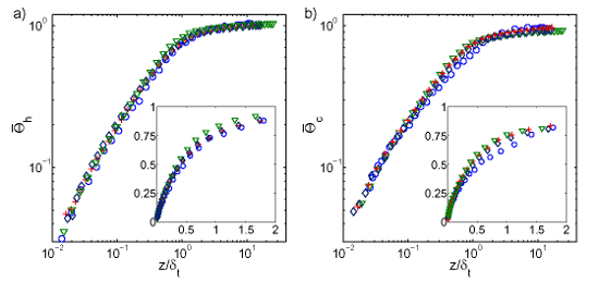
A selection of the normalized mean temperature profiles at aspect ratios between \(\Gamma = 1.13\) and \(7.00\) are plotted in figure 3. All profiles obtained at one plate turn out to be similar, with the deviation not exceeding 10%. Small deviations visible in the lin-lin representation in the insets might be associated with non-Boussinesq effects due to the change in the temperature drop, which amounts to \(\Delta \theta = 2.4\) K in the experiment at \(\Gamma = 1.13\) and \(\Delta \theta = 45\) K in the \(\Gamma = 7.0\) experiment. While the variation of the fluid properties can be neglected for the minimum temperature difference, it is worth noting that, for example, the heat conductivity \(\lambda\) varies by about 15% across the cell for the highest one. This variation causes the temperature gradients at the surface of the heating and the cooling plates to differ by 15% as well.
 Fig. 3: Profiles of the normalized mean temperature at the heating (a) and at the cooling (b) plates for various aspect ratios G = 1.13 and Ra = 5.2E10 (○, blue), G = 2.00 and Ra = 5.3E10 (+, red), G = 4.00 and Ra = 3.9E9 (◇, black), and G = 7.00 and Ra = 3.8E9 (▽, green). The insets show the region within the boundary layer in a lin-lin representation.
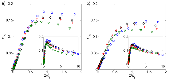
The profiles of the root-mean-square (rms) temperature fluctuations, expressed as \[\sigma(z) = (2/\Delta T) \{ [1/(N-1)] \sum_i [T_i(z) - \overline{T}(z)]^2\}^{1/2}\] where \(\overline{T}(z)\) is the mean temperature, are shown in figure 4, in order to see whether they remain unchanged with increasing the aspect ratio as well. The gradient \(\partial \sigma/\partial (z/\delta_t)\) remains constant up to 70% of the maximum of the fluctuations and is virtually equal for all aspect ratios. The position of the maxima coincides fairly well with \(z /\delta_t = 1\), supporting the assumption that the displacement thickness is a well-suited basis to judge about the conservation of the typical flow field. The position of the maxima corresponds as well with the position where about 70% of the maximum temperature drop across the boundary layer is reached, which is in good agreement with early measurements in water reported by Tilgner et al (1993) and Lui and Xia (1998).
 Fig. 4: Profiles of the root-mean-square (rms) temperature fluctuations at the heating (a) and at the cooling (b) plates for various aspect ratios G = 1.13 and Ra = 5.2E10 (○, blue), G = 2.00 and Ra = 5.3E10 (+, red), G = 4.00 and Ra = 3.9E9 (◇, black), and G = 7.00 and Ra = 3.8E9 (▽, green). The insets show the entire domain.
References
- du Puits, R., Resagk, C., Thess, A. (2013). Thermal boundary layers in turbulent Rayleigh-Bénard convection at aspect ratios between 1 and 9. New J. Phys., Vol. 15, p. 013040.
- du Puits, R., Resagk, C., Thess, A. (2007a). Breakdown of wind in turbulent thermal convection. Phys. Rev. E, Vol. 75, p. 016302.
- Tilgner, A., Belmonte, A., Libchaber, A. (1993). Temperature and velocity profiles of turbulent convection in water. Phys. Rev. E, Vol. 47, p. 2253.
- Lui, S-L., Xia, K.-Q. (1998). Spatial structure of the thermal boundary layer in turbulent convection. Phys. Rev. E, Vol. 57, p. 5494.
- du Puits, R., Resagk, C. Tilgner, A., Busse, F. H., Thess, A.. (2007b) Structure of thermal boundary layers in turbulent Rayleigh-Bénard convection. J. Fluid Mech., Vol. 572, pp. 231-254.
Acknowledgements
The authors gratefully acknowledge the financial support for their research work from the German Science Foundation (DFG) under grant number TH 497/22-1 and the Ministry of Education and Culture, Thüringer, Germany.
Indexed data:
| case091 (dbcase, confined_flow) | |
|---|---|
| case | 091 |
| title | Thermal boundary layers in turbulent Rayleigh-Benard convection at aspect ratios between 1 and 9 |
| author | du Puits, Resagk, Thess |
| year | 2013 |
| type | EXP |
| flow_tag | 3d, scalar, buoyant |