Table of Contents
Viscous Boundary Layers in Turbulent Rayleigh-Bénard Convection
Experiments and DNS by Li, Resagk, du Puits, Shi, Emran, Schumacher and Thess
Description
The velocity field has been studied in a large-scale Rayleigh-Bénard (RB) experiment (called “Barrel of Ilmenau”, see also cases 91, 94 and 95) meeting two important criteria: a very high Rayleigh number of \(Ra_{max} = 10^{12}\) and a large size of 7.15 m in diameter and 6.30 m in height. The dynamics of the flow in a cylindrical RB cell is determined by three input parameters: the Rayleigh number \(Ra = (\gamma g \Delta \theta H^3)/(\nu k)\), the Prandtl number \(Pr = \nu/k\), and the aspect ratio \(\Gamma = D/H\). Its response to the applied temperature difference is reflected by the global output parameters: Reynolds number \(Re = (v_m H)/\nu\) and Nusselt number \(Nu = (4Hq)/(\lambda \pi D^2\Delta \theta)\). In these definitions variables stand for the following physical quantities: \(\gamma\) - isobaric expansion coefficient, \(g\) - gravitational acceleration, \(\Delta \theta\) - temperature difference between both horizontal plates, \(\nu\) - kinematic viscosity, \(k\) - thermal diffusivity, \(D\) - diameter of the cell, \(H\) - plate distance, \(v\) - typical velocity, \(q\) - convective heat flux, and \(\lambda\) - thermal conductivity.
Highly resolved local velocity and temperature profiles inside the boundary layers in turbulent Rayleigh-Bénard convection in air are presented. All component profiles were performed in a cylindrical box with an aspect ratio \(\Gamma = 1\), a Prandtl number \(Pr = 0.7\) and Rayleigh numbers \(Ra = 3 \times 10^9\) and \(Ra = 3 \times 10^{10}\). The experimentally obtained velocity profiles are compared with data from Direct Numerical Simulations (DNS) at the same Rayleigh numbers. The profiles of mean velocity from both experiments and numerics collapse very well with each other and both of the mean horizontal velocity profiles differ from the Blasius solution of a laminar non-isothermal shear layer. The wall-normal mean velocity at the central window tends to zero in both experiment and DNS. The temperature was measured by a very small glass encapsulated micro-thermistor of a size 125 \(\mu\)m. It should be noted that the typical thickness of the boundary layers is of order of 10 mm at the Rayleigh numbers covered in this work. Each single measurement covers the distance between z = 70 \(\mu\)m (corresponding to half the diameter of the micro-thermistor) and z = 150 mm.
Measurement and DNS details
Experimental details
A sketch of the experimental facility is shown in figure 1. In order to match the experimental parameters to those from the DNS (\(Ra_{sim} = 3 \times 10^9\), \(Ra_{sim} = 3 \times 10^{10}\)) a smaller cell, with a diameter of 2.5 m and a height of 2.5 m, was installed in the large RB system. Four windows are located at several positions of the cooling plate, permitting optical access for the Laser Doppler Anemometer (LDA) measurement. Using a combination of a 2d- and a 1d-Laser Doppler Anemometer (LDA), highly resolved profiles of the velocity were measured (see figure 2).
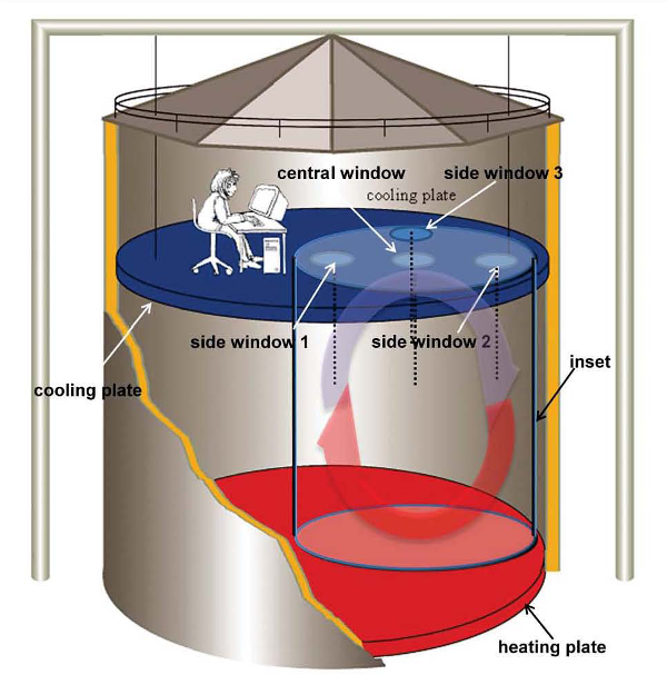 Fig. 1: Sketch of the large-scale experiment "Barrel of Ilmenau"
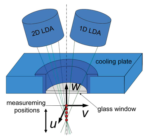 Fig. 2: Set-up of the 3d-Laser Doppler anemometry measurement
The probes were arranged above the various windows in the cooling plate to provide field information at different locations in the flow. They are mounted on a high precision traverse system, which could be moved in the vertical \(z\)-direction in steps of \(\Delta z = 0.01\) mm. By moving the probes up and down the velocity could be measured at different locations beneath the plate surface. At each position different time series of 1800 s, 3600 s, 7200 s were captured and analyzed. Typical data rates were of the order of 100 Hz on average, which was sufficiently high to resolve the fastest velocity fluctuations in the flow. Cold-atomized droplets of Di-Ethyl-Hexyl-Sebacat (DEHS) with a size of about 1 \(\mu\)m were used as tracer particles, which were injected through an opening close to the sidewall. Because of the oscillation of large-scale circulation in turbulent RB convection, the magnitude \(U =(U^2 + V^2)^{1/2}\) is taken as the mean horizontal velocity. The actual set-up permits the measurement of the wall-normal velocity component, \(w\), up to a distance of 200 mm away from the wall.
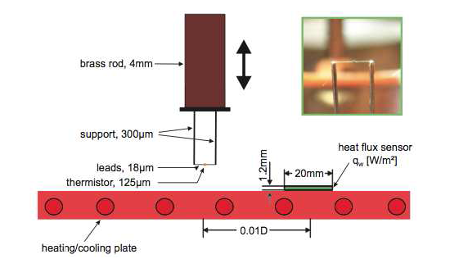
For the temperature measurement set-up (see figure 3), the thermistor is connected to the tips of two 0.3 mm supports by 18 \(\mu\)m wires. In order to reduce the measurement error the temperature sensor was redesigned, taking care that the connecting wires were aligned parallel to the plates and along the iso-surfaces of constant mean temperature in the flow. The measurement uncertainty of the RTD is specified with 0.02 K in the range between 0 and 100 degrees. The micro-thermistor is connected to a special resistance bridge with an internal amplifier providing a very low current of ITh = 5 \(\mu\)m, which is sufficiently small to keep the self-heating of the sensor as low as 10 mK. The bridge was connected to a PC based multi-channel data acquisition system with a resolution of 10-4 K and a sampling rate of 200 s-1.
Direct numerical simulation details
A three-dimensional Direct Numerical Simulation (DNS) was used, with the Boussinesq approximation, which incorporates the effect of temperature in the vertical direction only. Owing to the cylindrical geometry cylindrical coordinates were employed, (\(r, \phi, z)\). Boundary conditions were the no-slip condition for the velocity at all walls, isothermal top and bottom plates, and adiabatic side walls for the temperature.
The grid sizes were \(N_r \times N_{\phi} \times N_z = 301 \times 513 \times 360\) for \(Ra = 3 \times 10^9\) and \(513 \times 1153 \times 861\) for \(Ra = 3 \times 10^{10}\) . The DNS scheme by Verzicco and Orlandi (1996) was used, in which equations are solved on a staggered grid with a second-order finite difference scheme. The pressure field \(p\) was determined by a two-dimensional Poisson solver after applying a one-dimensional Fast Fourier Transform (FFT) in the azimuthal direction. The time advancement was done by a third-order Runge-Kutta scheme. The grid spacings were non-equidistant in the axial and radial directions. The grid resolutions were chosen sufficiently large (see Shi et al (2012) for more details), and ensured that the thermal boundary layer was resolved with 18 grid planes for the \(Ra = 3 \times 10^9\) case and with 23 grid planes for the \(Ra = 3 \times 10^{10}\) case.
In order to compare the results with the experiments in “Barrel of Ilmenau” the same measurement procedure was followed, by taking time series of the turbulent fields at several locations in the cell, which allowed wall-normal mean profiles of the turbulent fields to be determined. For the lower Rayleigh number case there were four arrays containing 40 measurement points each. They were seeded in order to track fully resolved time series of the three velocity components and the temperature. Probe arrays were positioned as in the experiment. There were 100 measurement points for the larger Rayleigh number run.
Available Data
Data available includes:
- Mean and rms velocity and temperature profiles across the boundary layers on the cold plate
- Dynamic and thermal boundary layer thicknesses for a range of Rayleigh numbers
- Shear Reynolds number for a range of Rayleigh numbers
Sample plots of selected quantities are available.
The data files can be downloaded as compressed archives, or individually from the tables below (data are available in both plain text files and Excel spreadsheets).
| Experimental | DNS | Excel sheet (with both experimental and DNS) | |
|---|---|---|---|
| Boundary layer thicknesses | exp-blthickness.dat | dns-blthickness.dat | thickness_of_boundary_layers.xlsx |
| Shear Reynolds numbers | exp-shear-re.dat | dns-shear-re.dat | shear_reynolds_numbers.xlsx |
Discussion of Results
The graphs in figure 4 show the mean and rms horizontal velocity profiles at the centerline of the cylinder, normalized by the maximum values. In both cases, the near-wall part of the profiles grows almost linearly and coincides with the Prandtl-Blasius solution, as visible in the inset of figure 4(a) and (b). At larger distances from the wall the profiles noticeably start to deviate from the theoretical prediction of the laminar shear layer, especially for the velocity at the lower \(Ra\). We can thus conclude that the Blasius profile cannot perfectly describe the profiles of the mean velocity in turbulent RB convection for the range of Rayleigh numbers which is accessible in the measurements and simulations. The standard deviation (or root-mean-square) of the horizontal velocity, \(\sigma_U (z)\), which are normalized by \(\sigma_{max}\), are shown in figure 4(c), (d). The comparison of the data at \(Ra = 3 \times 10^9\) and \(Ra = 3 \times 10^{10}\) indicates a very good agreement except for a minor departure in the measured profile at the higher \(Ra\). The local maximum of the profile is for both cases at about the same distance from the wall, although the BL gets finer as \(Ra\) increases.
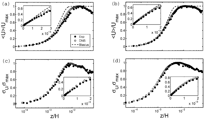 Fig. 4: Profiles of the mean horizontal velocity (a, b) and the standard deviation (c, d) measured in the experiment (closed circles) and obtained from the DNS (open circles) at the lower (a, c) and and higher (b, d) Rayleigh number. The dashed lines in (a) and (b) represent the velocity field of a laminar flat plate BL according to Prandtl-Blasius. The insets show the near-wall region of the BL.
The mean profiles of the wall-normal velocity component are plotted in figure 5(a), (b). In order to show that the mean wall-normal component velocity is much smaller than the mean horizontal component velocity, they are normalized by the maximum mean horizontal velocity \(U_{max}\). The good agreement between the measured data and the DNS data indicates that the mean wall-normal velocities tend to zero, namely, there is no mean vertical velocity on the centreline. This result is in agreement with the PIV measurements by Sun et al. (2008). As can also be seen, from figure 5(c), (d), the wall-normal standard deviations are not zero, and the the fluctuations of the vertical velocity component start to increase rapidly at the edge of the BL.
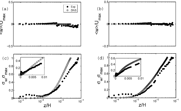 Fig. 5: Profiles of the wall-normal velocity (a, b) and the standard deviation (c, d) measured in the experiment (closed circles) and obtained from the DNS (open circles) at the lower (a, c) and higher (b, d) Rayleigh numbers. The insets show the near-wall region of the BL.
Turning to the mean temperature profiles which are displayed in figure 6(a) and (b), normalized by the difference between the bulk temperature and cooling plate temperature, the agreement between the measurement and the numerical data is not as perfect as for the velocity data, but still satisfactory. A very detailed view close to the plate surface, however, shows that the temperature gradient at the wall obtained in the measurements differs from that computed in the DNS data (see insets of figure 6(a) and (b)). It exceeds that obtained from the DNS by a factor of 2.5 at \(Ra = 3 \times 10^9\) and by a factor of 1.5 at \(Ra = 3 \times 10^{10}\). In other words, the local heat flux in the experiment is 2.5 (1.5) times larger than the numerical one. Currently, the conclusive explanation for this difference is not known. The standard deviation of the temperature, \(\sigma_T (z)\), normalized by its maximum maximum value \(\sigma_{max}\), is plotted in figure 6(c) and (d). It can be seen that this has the same trend in both cases. At \(Ra = 3 \times 10^9\), the temperature fluctuations have 10 ~ 20% difference from each other before they approach their maximum value; for larger distances away from the wall the difference decreases to about 5%. At \(Ra = 3 \times 10^{10}\) the fluctuations agree with each other, especially up to the maximum fluctuation point. For larger \(z\), there is a difference of about 10% in comparison to the DNS.
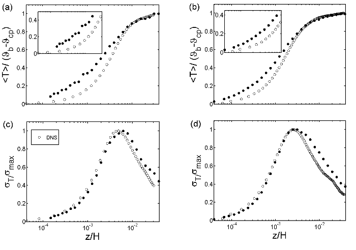 Fig. 6: Profiles of the mean temperature (a, b) and the standard deviation (c, d) measured in the experiment (closed circles) and obtained from the DNS (open circles) at the lower (a, c) and higher (b, d) Rayleigh numbers. The insets show the near-wall region of the BL.
In RB cells of aspect ratio one and smaller the sidewalls can significantly affect the flow inside the enclosure. Therefore, it is justified to ask whether or not the results obtained at the center of the cooling plate can be generalized to the entire area? First, the experimental and DNS mean horizontal velocity profiles at \(Ra = 3 \times 10^{10}\) are presented in figure 7(a) and (b). In order to show any potential deviation from the profile at the central axis the velocity is normalized by the same value \(U_{max}\) as used in figure 4 and figure 5. The maximum of the velocity at the outer positions is significantly below the value at the centreline. This implies a reduction of the local heat transfer coefficient and, hence, a decrease of the local \(Nu\). All three measured profiles rise with a different gradient toward their maximum, and the thickness of the viscous BL varies. Unlike on the central axis of the experiment, the mean wall-normal velocities at windows 1 and 2 (begin and end of the path of the LSC along the cooling plate) clearly deviate from zero. In the area of up-welling plumes (1) a positive \(W\) component has been measured, while this velocity component is negative in the area of down-welling plumes. At window 3, which is outside the LSC, the mean of \(W\) tends to zero. Since in the DNS areas of up- and down-welling plumes are not assigned with distinct positions at the cooling plate the observed effect is weaker, but clearly visible too (see figure 8(b)).
 Fig. 7: Mean horizontal velocity profiles at side windows 1, 2 and 3 at the higher Ra. (a) Profiles of the measured data at window 1 (circle), window 2 (triangle) and window 3 (star). (b) Profiles of the DNS data at window 1 (circle), window 2 (triangle) and window 3 (star).
 Fig. 8: Mean wall-normal velocity profiles at side windows 1, 2 and 3 at the higher Ra. (a) Profiles of the measured data at window 1 (circle), window 2 (triangle) and window 3 (star). There is a clear pair of upwelling and downwelling mean velocities. (b) Profiles of the numerical data at window 1 (circle), window 2 (triangle) and window 3 (star).
In figure 9 the obtained BL thickness values versus the corresponding Rayleigh numbers in a range between \(Ra = 10^9\) to \(Ra = 10^{12}\) are summarized. It was found that the viscous BL thickness scales with the \(Ra\) as \(\delta_v/H \approx 0.66 Ra^{-0.24}\), i.e., with the same exponent as predicted by Grossmann and Lohse (2000). The local thickness of the thermal BL on the centreline is found to scale with respect to \(Ra\) as \(\delta_{\theta}/H \approx 0.76Ra^{-0.24}\).
 Fig. 9: Thickness of the viscous (a) and the thermal (b) boundary layers versus Ra. Experimental results are displayed as closed symbols, DNS data points are open symbols. The solid lines in each of the graphs correspond to the power laws given in the text\(\delta_v / H = 0.66 Ra^{-0.24}\) and \(\delta_{\theta} / H = 0.76 Ra^{-0.24}\), respectively.
In figure 10 the shear Reynolds number is plotted in a range between \(Ra = 10^9\) to \(Ra = 10^{12}\). \(Re_s\) increases monotonically with \(Ra\) and, again, experimental and numerical data fit very well. In order to estimate the \(Ra\) numbers at which the trend crosses the critical limits \(Re_s = 320\) or \(Re_s \approx 420\) the data points were extrapolated using a regression \(Re_s \propto Ra^{0.267 \pm 0.0386}\). According to this fit the lowest possible \(Ra\) for a transition to a turbulent state amounts to \(Ra_c \approx 2 \times 10^{12}\), which would be below the prediction of Grossmann and Lohse (2000) and the recent experimental findings by Funfschilling and Ahlers (2004). However, it cannot be ruled out that due to the plume inside the BLs, as well as the strongly three-dimensional flow in turbulent RB convection, and the complex dynamics of the LSC, this transition may take place at even lower Rayleigh numbers.
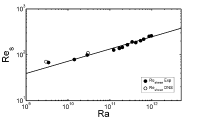 Fig. 10: Shear Reynolds number Res versus Ra from experiment (closed circles) and DNS (open circles). The solid line is the fit to all data.
References
- du Puits, R., Resagk, C., Thess, A. (2009). Structure of viscous boundary layers in turbulent Rayleigh-Bénard convection. Phys. Rev. E, Vol. 80, p. 036318.
- Funfschilling, D., Ahlers, G. (2004). Plume motion and large-scale circulation in a cylindrical Rayleigh–Bénard cell. Phys. Rev. Lett., Vol. 92, p. 194502.
- Grossmann, S., Lohse, D. (2000). Scaling in thermal convection: a unifying theory. J. Fluid Mech., Vol. 407, pp. 27–56.
- Li, L., Resagk, C., du Puits, R. (2011). Viscous boundary layers in turbulent Rayleigh-Bénard convection. Journal of Physics: Conference Series, Vol. 318, p. 082004.
- Li, L., du Puits, R. (2012). 3-d measurements of the velocity in the boundary of turbulent convection. Springer Proceedings in Physics, Vol. 141, p. 283.
- Li, L., Shi, N., du Puits, R., Resagk, C., Schumacher, J., Thess, A. (2012). Boundary layer analysis in turbulent Rayleigh-Bénard convection in air: experiment versus simulation. Phys. Rev. E, Vol. 86, p. 026315.
- Shi, N., Emran, M.-S., Schumacher, J. (2012). Boundary layer structure in turbulent Rayleigh-Bénard convection. J. Fluid Mech., Vol. 706, p. 5.
- Sun, C., Cheung, Y. H., Xia, K. (2008). Experimental studies of the viscous boundary layer properties in turbulent Rayleigh-Bénard convection. J. Fluid Mech., Vol. 605, p. 79.
- Verzicco, R., Orlandi, P. (1996). A finite-difference scheme for three-dimensional incompressible flows in cylindrical coordinates. J. Comput. Phys., Vol. 123, pp. 402–414.
Acknowledgements
The authors gratefully acknowledge the financial support for their research work from the German Science Foundation (DFG), Germany, FOR 1182 - DFG Research Unit: Transport and structure formation in turbulent Rayleigh-Bénard-, Taylor-Couette- and pipe flows near solid walls.
Indexed data:
| case090 (dbcase, confined_flow) | |
|---|---|
| case | 090 |
| title | Viscous boundary layers in turbulent Rayleigh-Benard convection |
| author | Li, Resagk, du Puits, Shi, Emran, Schumacher, Thess |
| year | 2012 |
| type | EXP |
| flow_tag | axisymmetric, scalar, buoyant |
